blog
Distributed Machine Learning Framework
Partition&Parallelism
Data Parallelism
Data parallelism focuses on distributing the data across different nodes, which operate on the data in parallel. There are two ways to split data: split samples(random sampling/shuffling and dividing as mini-batch) and split dimensions(only used in dimensions that are mutually independent).
Model Parallelism
Linear Model
Linear models like Linear Regression or Logistic Regression have the same size of parameters as the size of dimensions and the dimensions are mutually independent (like what we mention in data parallelism). We can divide the dimensions and use coordinate descent method to optimize the model.
Neural Network
Divide the model into different parts and allocate the task to different nodes. Every divided node would calculate the output after all of the node’s dependences are calculated then update the parameters and send output to the next node.
Horizontal Partition(also can be called workload parallelism)
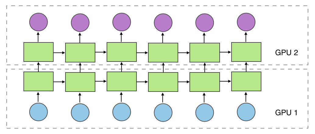
It partitions workload in different layers into different part (not only allocated in GPU).
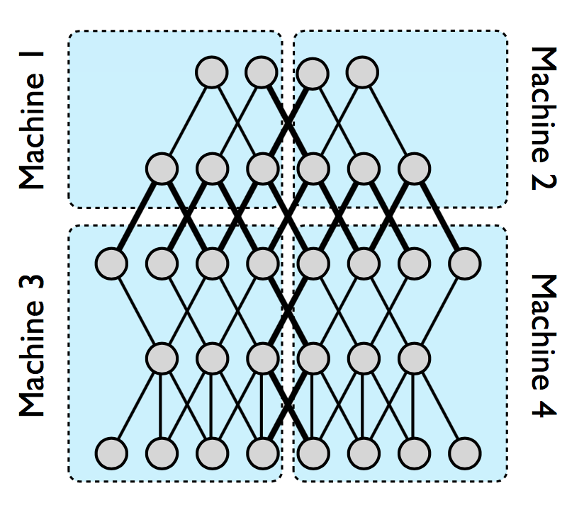
Vertical Partition
It partitions workload in vertical into different part (e.g. group convolution).
Mixed Partition
Put horizontal partition and vertical partition together. (e.g. DistBelief[1])
Random Partition
Explore the optimal partition for neural network, mainly used in model compression.
Distributed Computing Model
Data/Model Parallelism
MapReduce/AllReduce[2]
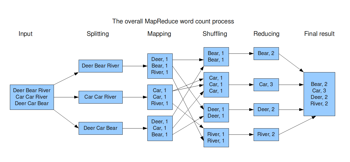
A MapReduce framework (or system) is usually composed of three operations (or steps):
- Map: each worker node applies the
mapfunction to the local data, and writes the output to a temporary storage. A master node ensures that only one copy of the redundant input data is processed. - Shuffle: worker nodes redistribute data based on the output keys (produced by the
mapfunction), such that all data belonging to one key is located on the same worker node. - Reduce: worker nodes now process each group of output data, per key, in parallel.
When synchronizing clusters in MapReduce framework, we can use MPI(Message Passing Interface) like AllReduce.
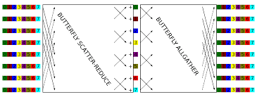
e.g. Hadoop, Spark
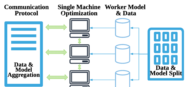
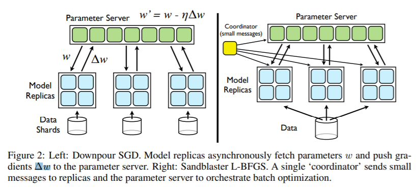
Parameter Server[3]
If one node in MapReduce doesn’t work, the whole system would stop. The parameter server makes all the parameter in one server. The workers only communicate with server and there is no need for workers to communicate with each other.
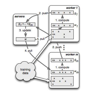
e.g. Multiverso
Streaming
Conceptually, a stream is a (potentially never-ending) flow of data records, and a transformation is an operation that takes one or more streams as input, and produces one or more output streams as a result.
e.g. Flink
Dataflow(Many can be accounted as this)
dataflow programming is a programming paradigm that models a program as a directed graph of the data flowing between operations, thus implementing dataflow principles and architecture. Here we specify this as dataflow and differentiable programming, which means that every node in dataflow is responsible only for forward computing but also for backward computing.
e.g. Pytorch
Concurrent Design Pattern
Many distributed design patterns are borrowed from this.
Master/Worker(can be seen as Map-Reduce)
This pattern can be used when data can be divided into multiple parts, all of which need to go through the same computation to give a result, which need to be aggregated to get the final result.
Async Method Invocation
Also see Asynchronous Communication
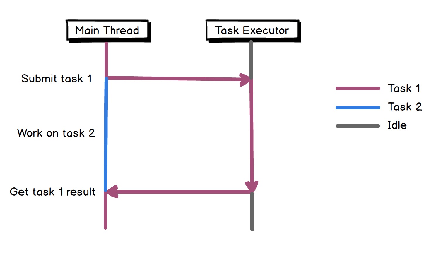
e.g. Future/Promise
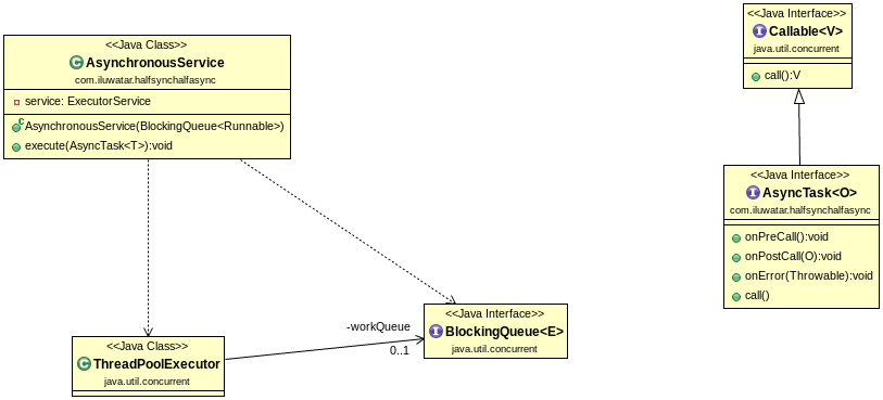
Half-Sync/Half-Async
The Half-Sync/Half-Async pattern decouples synchronous I/O from asynchronous I/O in a system to simplify concurrent programming effort without degrading execution efficiency.
Concurrent Communication Model
Actor
Actors are concurrency primitives which can send messages to each other, create new Actors and determine how to respond to the next received message. They keep their own private state without sharing it, so they can affect each other only through messages. Since there is no shared state, there is no need for locks.
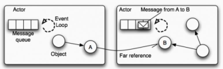
e.g. Akka
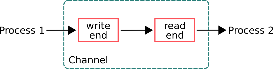
CSP
Communicating Sequential Processes (CSP) is a paradigm which is very similar to the Actor model. It’s also based on message-passing without sharing memory. However, CSP and Actors have these 2 key differences:
- Processes in CSP are anonymous, while actors have identities. So, CSP uses explicit channels for message passing, whereas with Actors you send messages directly.
- With CSP the sender cannot transmit a message until the receiver is ready to accept it. Actors can send messages asynchronously.
STM
While Actors and CSP are concurrency models which are based on message passing, Software Transactional Memory (STM) is a model which uses shared memory. It’s an alternative to lock-based synchronization. Similarly to DB transactions, these are the main concepts:
- Values within a transaction can be changed, but these changes are not visible to others until the transaction is committed.
- Errors that happened in transactions abort them and rollback all the changes.
- If a transaction can’t be committed due to conflicting changes, it retries until it succeeds.
Communication
Method
RPC/HTTP/MQ/Socket/…
Pace
Synchronous Communication
BSP
Bulk Synchronous Parallel computer consists of
- components capable of processing and/or memory transactions,
- a network that routes messages between pairs of such components, and
- a hardware facility that allows for the synchronisation of all or a subset of components.
In distributed model, the BSP model can not only be run on multiple processors(CPU, GPU, etc.), but also can be allocated in multiple servers.
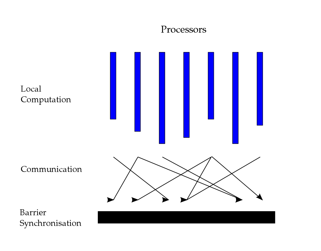
e.g. Pregel
Asynchronous Communication
See Distributed Machine Learning Algorithms
SSP(Stale Synchronous Parallel)
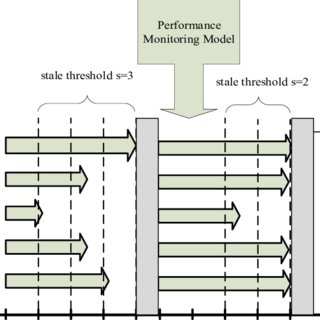
Tackle the difference of pace of worker in asynchronous communication.
Aggregation
We consider two ways of aggregation of model parameters:
- All parameters/output adding. This is mainly for data parallelism. e.g. MA, ADMM, SSGD, etc.
- Partial parameters/output adding. e.g. ASGD, AADMM, D-PSGD, etc.
See Distributed Machine Learning Algorithms
Distributed Machine Learning Algorithms
| Algorithm | Parallelism | Communication | Aggregation |
|---|---|---|---|
| SSGD | data | sync | all |
| MA | data | sync | all |
| BMUF | data | sync | all |
| ADMM | data | sync | all |
| EASGD | data | sync | all |
| ASGD | data | async | partial |
| AADMM | data | async | partial |
| Hogwild! | data | async | partial |
| Cylades | data | async | partial |
| D-PSGD | data | async | partial |
| AdaDelay | data | async | partial |
| Group Convolution | model | sync | all |
| DistBelief | model | async | partial |
Synchronous Algorithm
SSGD
Initialize: parameter w_0, number of workers K, epochs T, learning rates \eta
for t = 0, 1, ..., T - 1:
    Pull w_t
    Random sampling mini-batch data i
    Calculate gradient \Delta f_i(w_t)
    Get all gradients in workers and get \sum \Delta f_i(w_t)
    Update w_{t+1} = w_t - \eta/K \sum \Delta f_i(w_t)
This method is suit for big computation of every mini-batch. If the batch is too small it would cost a lot of time to communicate. Also, the optimal batch size of neural network is not determined. If we want to use SSGD for optimization, we should consider the trade-off between time and accuracy.
MA
Initialize: parameter w_0, number of workers K, epochs T, gapping M, learning rates \eta
for t = 0, 1, ..., T - 1:
    Pull w_t
    for m = 0, 1, ... M:
    	Random sampling mini-batch data i_m
    	Calculate gradient \Delta f_i_m(w_t)
    	Update w_t = w_t - \eta \Delta f_i_m(w_t)
    Get all parameters in workers and get 1/K \sum w_t
    Update w_{t+1} = 1/K \sum w_t
e.g. CNTK
BMUF
Adding a global momentum
Initialize: parameter w_0, number of workers K, epochs T, gapping M, learning rates \eta, momentum \mu, \delta
for t = 0, 1, ..., T - 1:
    Pull w_t
    for m = 0, 1, ... M:
    	Random sampling mini-batch data i_m
    	Calculate gradient \Delta f_i_m(w_t)
    	Update w_t = w_t - \eta \Delta f_i_m(w_t)
    Get all parameters in workers and get \overline{w} = 1/K \sum w_t
    Compute \Delta_t = \mu \Delta_{t-1} + \delta (\overline{w} - w_t)
    Update  w_{t+1} = w_t + \Delta_t
ADMM
The problem of data parallelism distributed optimization can be described as:
ADMM introduces a variable z to control the difference among
, i.e. converting this problem as a constrained optimization problem
Thus, the optimization problem can be described as
Worker:
Initialize: parameter w_0^k, \lambda_t^k, number of workers K, epochs T
for t = 0, 1, ..., T - 1:
    Pull z_t
    Update \lambda_{t+1}^k = \lambda_t^k + \rho (w_t^k - z_t)
    Update w_{t+1}^k = argmin_w(\sum^K l^k(w^k) + (\lambda^k_t)^T (w^k-z_t) + \frac{\rho}{2} ||w^k-z_t||_2^2)
    Push w_{t+1}^k, \lambda_{t+1}^k
Master:
Initialize: parameter z_0, number of workers K
while True:
    while True:
    	Waiting w_{t+1}^k, \lambda_{t+1}^k
    	if received from all K workers: break
    Update z_{t+1} =  1/K \sum (w_t^k + \frac{1}{\rho} \lambda_t^k)
EASGD[4]
The constrained optimization problem in ADMM can be simplified as
we can take the first-order derivative in the update procedure.
Initialize: global parameter w_0, local parameter w_0^k, number of workers K, epochs T, learning rates \eta, constraint ratio \alpha, \beta
for t = 0, 1, ..., T - 1:
   Random sampling mini-batch data i
   Calculate gradient \Delta f_i(w_t)
   Update w_{t+1}^k = w_t^k - \eta \Delta f_i(w_t^k) - \alpha(w_t^k - w_t)
   Get all parameters in workers and get 1/K \sum w_t
   Update global parameter w_{t+1} = (1-\beta)w_t + \beta/K \sum w_t
That is, when we update global parameters, we can take consideration of part of former parameters.
Asynchronous Algorithm
ASGD
Worker:
Initialize: parameter w_0, number of workers K, epochs T, learning rates \eta
for t = 0, 1, ..., T - 1:
    Pull w_t^k
    Random sampling mini-batch data i
    Calculate gradient g_t^k = \Delta f_i(w_t)
    Push g_t^k
Master(PS):
while True:
    while True:
        if received g_t^k:
        break
    Update w = w - \eta g_t^k
It’s very easy to get delay in this algorithm. The update formula can also be written as
This would make the training unstable and may produce inaccurate result.
AADMM
Worker:
Initialize: parameter w_0^k, \lambda_t^k, number of workers K, epochs T
for t = 0, 1, ..., T - 1:
    Pull z_t
    Update \lambda_{t+1}^k = \lambda_t^k + \rho (w_t^k - z_t)
    Update w_{t+1}^k = argmin_w(\sum^K l^k(w^k) + (\lambda^k_t)^T (w^k-z_t) + \frac{\rho}{2} ||w^k-z_t||_2^2)
    Push w_{t+1}^k, \lambda_{t+1}^k
Master(PS):
Initialize: parameter z_0, number of workers K, max delay worker K_0, max delay \tau
while True:
    while True:
    	Waiting w_{t+1}^i, \lambda_{t+1}^i
    	if received from worker set \Phi(which contains no less than K_0 workers) and max(\tau_1, \tau_2, ..., \tau_K_0) \le \tau: break
    for i in \Phi:
         \tau_i = 1
    for i not in \Phi:
         \tau_i = \tau_i + 1
    Update z_{t+1} =  1/K \sum_{i \in \Phi} (w_t^i + \frac{1}{\rho} \lambda_t^i)
Hogwild![5]
Initialize: parameter w_0, learning rates \eta
while True:
    Random sampling mini-batch data i, using e representing the parameters related to i
    Calculate gradient g_j = \Delta_j f_i(w_t^j), j \in e
    Update w_t^j = w_t^j - \eta g_j
This is a lock-free asynchronous algorithm, which means that we don’t need to get the write permission of w. That’s because we can constraint the sparsity of loss function, i.e.
the smaller |e| and less intersection of e would make less conflicts when updating, and also guarantee the convergence of loss function.
Cyclades[6]
A significant benefit of the update partitioning in CYCLADES is that it induces considerable access locality compared to the more unstructured nature of the memory accesses during HOGWILD!
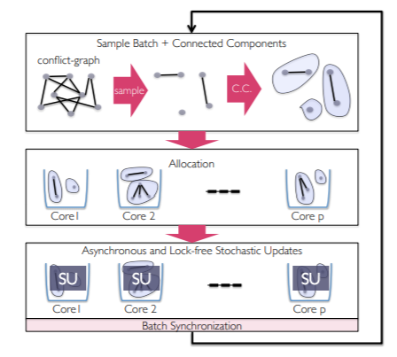
Initialize: Gu, T, B
Sample nb = T /B subgraphs G
Cores compute in parallel CCs for sampled subgraphs
for batch i:
    Allocation of C_i to P cores
    for each core in parallel:
        for each allocated component C:
            for each update j (in order) from C:
                x_j = u_j (x_j, f_j)
That is, predefine the subgraphs then compute.
D-PSGD[7]
This is also a decentralized algorithm like Cyclades etc.
Initialize: w_0^k, weight matrix W, learning rate \eta
for t = 0, 1, ..., T - 1:
     Random sampling mini-batch data i
     Calculate gradient g_t^k = \Delta f_i(w_t)
     Pull parameters from neighbors and get w^k_{t+1/2} = \sum_j W_k^j w_t^j
     Update w^k_{t+1} = w^k_{t+1/2} - \eta \Delta f_i(w_t)
AdaDelay[8]
This algorithm penalizes parameter updates when the nodes have delays. Assume the epoch is t and the delay is , then the step size
is
where
When
, the AdaDelay algorithm would become SGD with linear weight decay. In AdaDelay, the c is adaptive, i.e.
the weight average of historical gradient.
There some similar algorithms:
AsyncAdaGrad:
AdaptiveRevision:
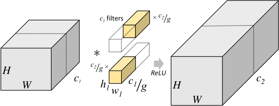
Group Convolution[9]
DistBelief[1]
Framework Based on MapReduce
Spark
RDD
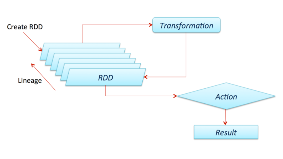
The main abstraction Spark provides is a resilient distributed dataset (RDD), which is a collection of elements partitioned across the nodes of the cluster that can be operated on in parallel. RDDs are created by starting with a file in the Hadoop file system (or any other Hadoop-supported file system), or an existing Scala collection in the driver program, and transforming it.
RDDs support two types of operations: transformations, which create a new dataset from an existing one, and actions, which return a value to the driver program after running a computation on the dataset. For example, map is a transformation that passes each dataset element through a function and returns a new RDD representing the results. On the other hand, reduce is an action that aggregates all the elements of the RDD using some function and returns the final result to the driver program (although there is also a parallel reduceByKey that returns a distributed dataset).
All transformations in Spark are lazy, in that they do not compute their results right away. Instead, they just remember the transformations applied to some base dataset (e.g. a file). The transformations are only computed when an action requires a result to be returned to the driver program. This design enables Spark to run more efficiently. For example, we can realize that a dataset created through map will be used in a reduce and return only the result of the reduce to the driver, rather than the larger mapped dataset.
Structured Streaming
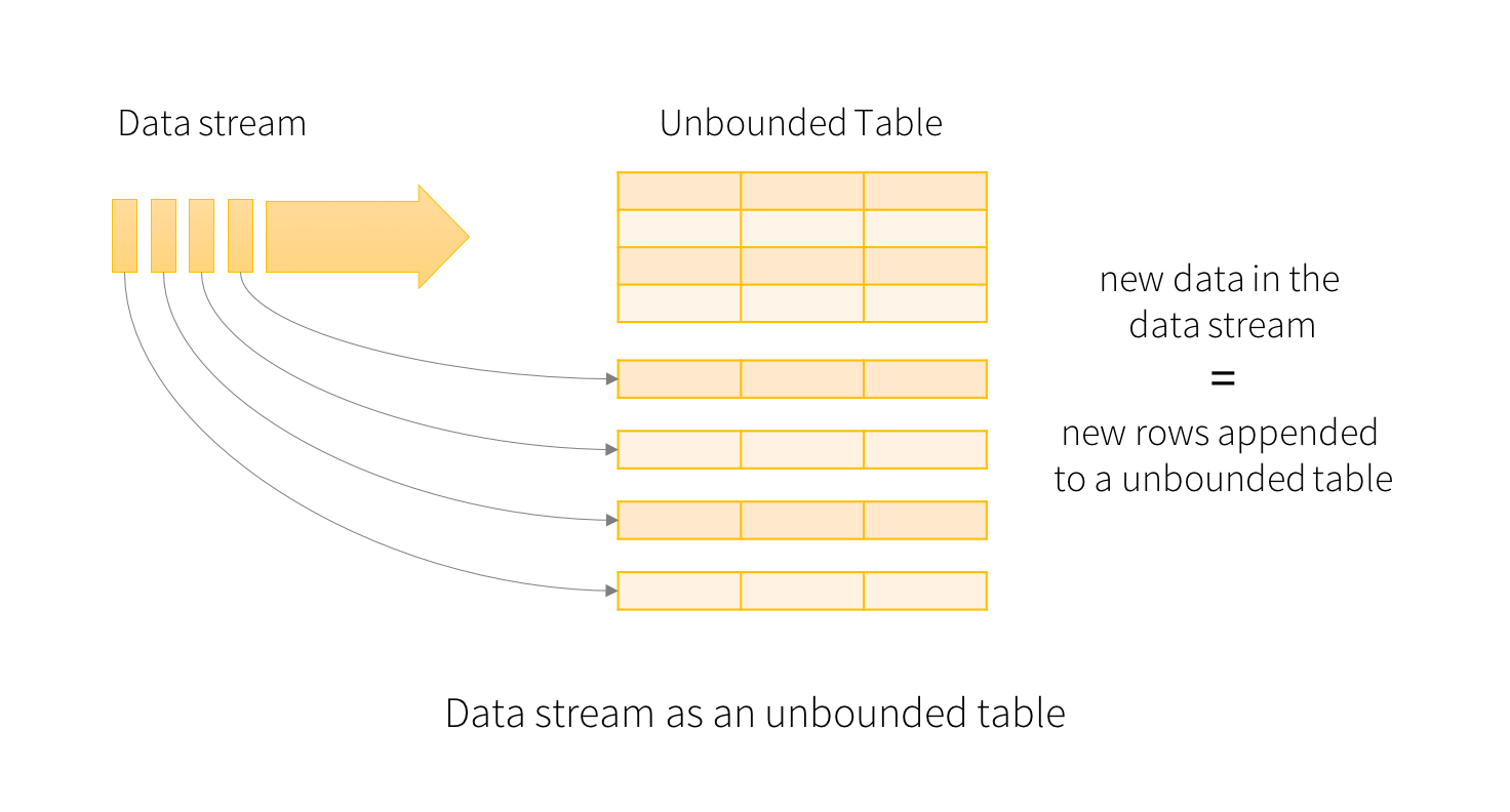
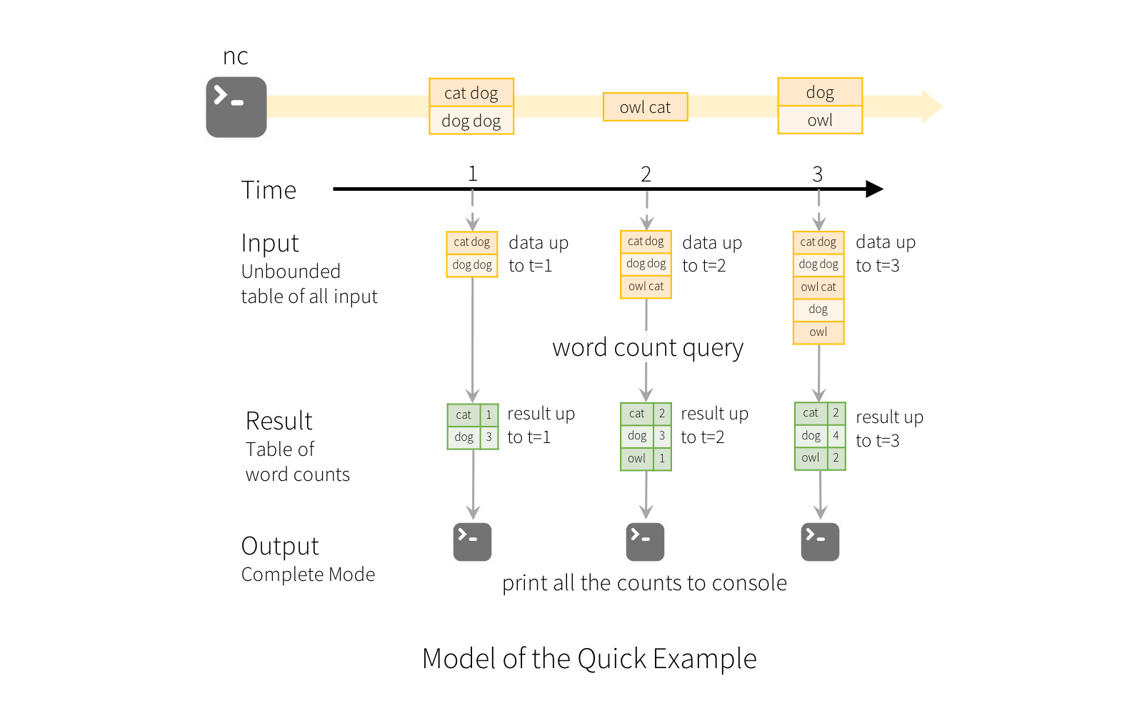
The key idea in Structured Streaming is to treat a live data stream as a table that is being continuously appended. This leads to a new stream processing model that is very similar to a batch processing model. You will express your streaming computation as standard batch-like query as on a static table, and Spark runs it as an incremental query on the unbounded input table. Let’s understand this model in more detail.
Distributed Components
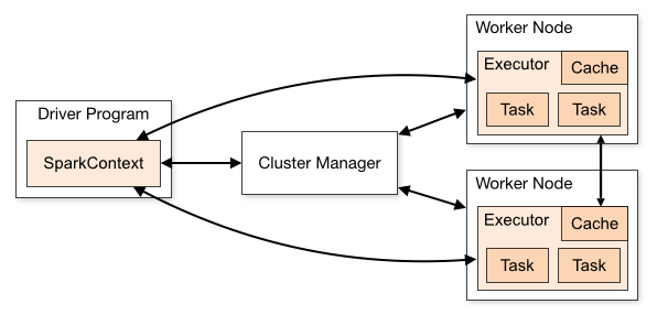
The SparkContext can connect to several types of cluster managers (either Spark’s own standalone cluster manager, Mesos or YARN), which allocate resources across applications. Once connected, Spark acquires executors on nodes in the cluster, which are processes that run computations and store data for your application. Next, it sends your application code (defined by JAR or Python files passed to SparkContext) to the executors. Finally, SparkContext sends tasks to the executors to run.
Framework Based on Differentiable Dataflow
TensorFlow
We mainly focus on TensorFlow2.
GradientTape
TensorFlow provides the tf.GradientTape API for automatic differentiation; that is, computing the gradient of a computation with respect to some inputs, usually tf.Variables. TensorFlow “records” relevant operations executed inside the context of a tf.GradientTape onto a “tape”. TensorFlow then uses that tape to compute the gradients of a “recorded” computation using reverse mode differentiation.
Graphs
Graphs are data structures that contain a set of tf.Operation objects, which represent units of computation; and tf.Tensor objects, which represent the units of data that flow between operations. They are defined in a tf.Graph context.
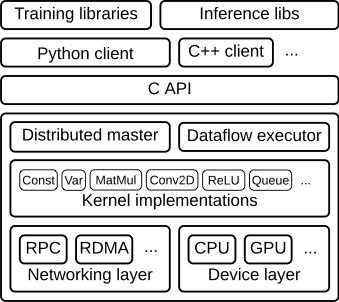
Architecture General View
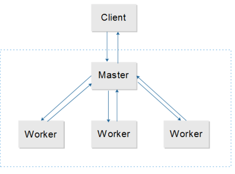
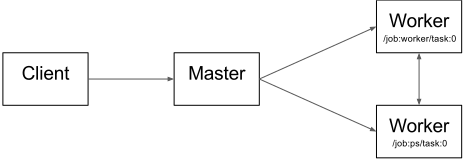
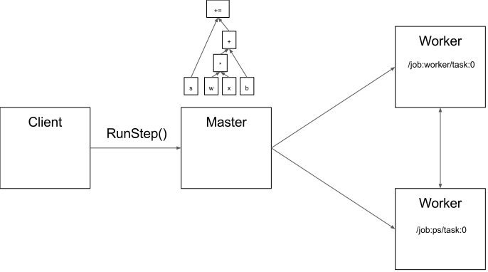
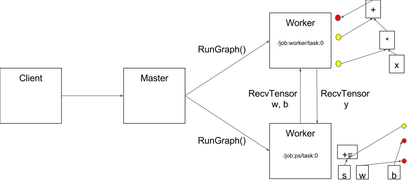
A general view of TensorFlow architecture can be seen as a Client-Master-Worker distributed architecture.
-
Client
The client creates a session, which sends the graph definition to the distributed master as a
tf.GraphDefprotocol buffer. When the client evaluates a node or nodes in the graph, the evaluation triggers a call to the distributed master to initiate computation. -
Distributed Master
- prunes the graph to obtain the subgraph required to evaluate the nodes requested by the client,
- partitions the graph to obtain graph pieces for each participating device, and
- caches these pieces so that they may be re-used in subsequent steps.
-
Worker Services
-
handles requests from the master,
-
schedules the execution of the kernels for the operations that comprise a local subgraph, and
-
mediates direct communication between tasks.
-
dispatches kernels to local devices and runs kernels in parallel when possible, for example by using multiple CPU cores or GPU streams.
-
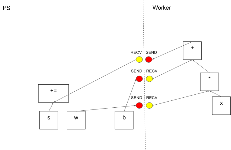
Send and Recv operations for each pair of source and destination device types:
- Transfers between local CPU and GPU devices use the
cudaMemcpyAsync()API to overlap computation and data transfer. - Transfers between two local GPUs use peer-to-peer DMA, to avoid an expensive copy via the host CPU.
For transfers between tasks, mainly uses multiple protocols, including:
- gRPC over TCP.(CPU&GPU)
- RDMA over Converged Ethernet.(GPUs)
- Transfers between local CPU and GPU devices use the
-
One way to enable workers is to allocate one for task and the other one for parameter storing and updating. This particular division of labor between tasks is not required, but is common for distributed training.
Between-Graph and In-Graph
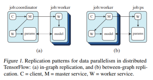
For in-graph replication (Figure 1(a)), a single client binary constructs one replica on each device (all contained in a massive multi-device graph), each sharing a set of parameters (resources) placed on the client’s own device. That clients master service then coordinates synchronous execution of all replicas: feeding data and fetching outputs. (Mainly used for one machine with many GPUs)
For between-graph replication (Figure 1(b)), multiple machines run a client binary, each creating a graph with a single replica on a local device, alongside resources on a shared device (i.e. the parameter server model). Because this relies on TensorFlows name resolution to share state, care must be taken to ensure each client creates resources identically.
Framework Containing Actor
Ray
Future
import ray
ray.init()

@ray.remote
def f(x):
    return x * x

futures = [f.remote(i) for i in range(4)]
print(ray.get(futures)) # [0, 1, 4, 9]
Actor
import ray
ray.init() # Only call this once.

@ray.remote
class Counter(object):
    def __init__(self):
        self.n = 0

    def increment(self):
        self.n += 1

    def read(self):
        return self.n

counters = [Counter.remote() for i in range(4)]
[c.increment.remote() for c in counters]
futures = [c.read.remote() for c in counters]
print(ray.get(futures)) # [1, 1, 1, 1]
Architecture
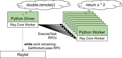
Task - A single function invocation that executes on a process different from the caller. A task can be stateless (a @ray.remote function) or stateful (a method of a @ray.remote class - see Actor below). A task is executed asynchronously with the caller: the .remote() call immediately returns an ObjectRef that can be used to retrieve the return value.
Object - An application value. This may be returned by a task or created through ray.put. Objects are immutable: they cannot be modified once created. A worker can refer to an object using an ObjectRef.
Actor - a stateful worker process (an instance of a @ray.remote class). Actor tasks must be submitted with a handle, or a Python reference to a specific instance of an actor.
Driver - The program root. This is the code that runs ray.init().
Job - The collection of tasks, objects, and actors originating (recursively) from the same driver.
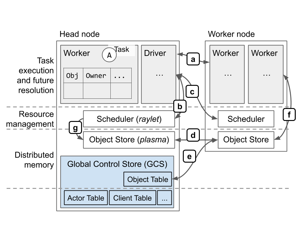
A Ray instance consists of one or more worker nodes, each of which consists of the following physical processes:
- One or more worker processes, responsible for task submission and execution. A worker process is either stateless (can execute any @ray.remote function) or an actor (can only execute methods according to its @ray.remote class). Each worker process is associated with a specific job. The default number of initial workers is equal to the number of CPUs on the machine. Each worker stores:
- An ownership table. System metadata for the objects to which the worker has a reference, e.g., to store ref counts.
- An in-process store, used to store small objects.
- A raylet. The raylet is shared among all jobs on the same cluster. The raylet has two main threads:
- A scheduler. Responsible for resource management and fulfilling task arguments that are stored in the distributed object store. The individual schedulers in a cluster comprise the Ray distributed scheduler.
- A shared-memory object store (also known as the Plasma Object Store). Responsible for storing and transferring large objects. The individual object stores in a cluster comprise the Ray distributed object store.
Each worker process and raylet is assigned a unique 20-byte identifier and an IP address and port. The same address and port can be reused by subsequent components (e.g., if a previous worker process dies), but the unique IDs are never reused (i.e., they are tombstoned upon process death). Worker processes fate-share with their local raylet process.
One of the worker nodes is designated as the head node. In addition to the above processes, the head node also hosts:
- The Global Control Store (GCS). The GCS is a key-value server that contains system-level metadata, such as the locations of objects and actors. There is an ongoing effort to support high availability for the GCS, so that it may run on any and multiple nodes, instead of a designated head node.
- The driver process(es). A driver is a special worker process that executes the top-level application (e.g.,
__main__in Python). It can submit tasks, but cannot execute any itself. Driver processes can run on any node, but by default are located on the head node when running with the Ray autoscaler.
Protocol overview (mostly over gRPC):
- a: Task execution, object reference counting.
- b: Local resource management.
- c: Remote/distributed resource management.
- d: Distributed object transfer.
- e: Location lookup for objects stored in distributed object store.
- f: Storage and retrieval of large objects. Retrieval is via
ray.getor during task execution, when replacing a task’s ObjectID argument with the object’s value. - g: Scheduler fetches objects from remote nodes to fulfill dependencies of locally queued tasks.
Ownership
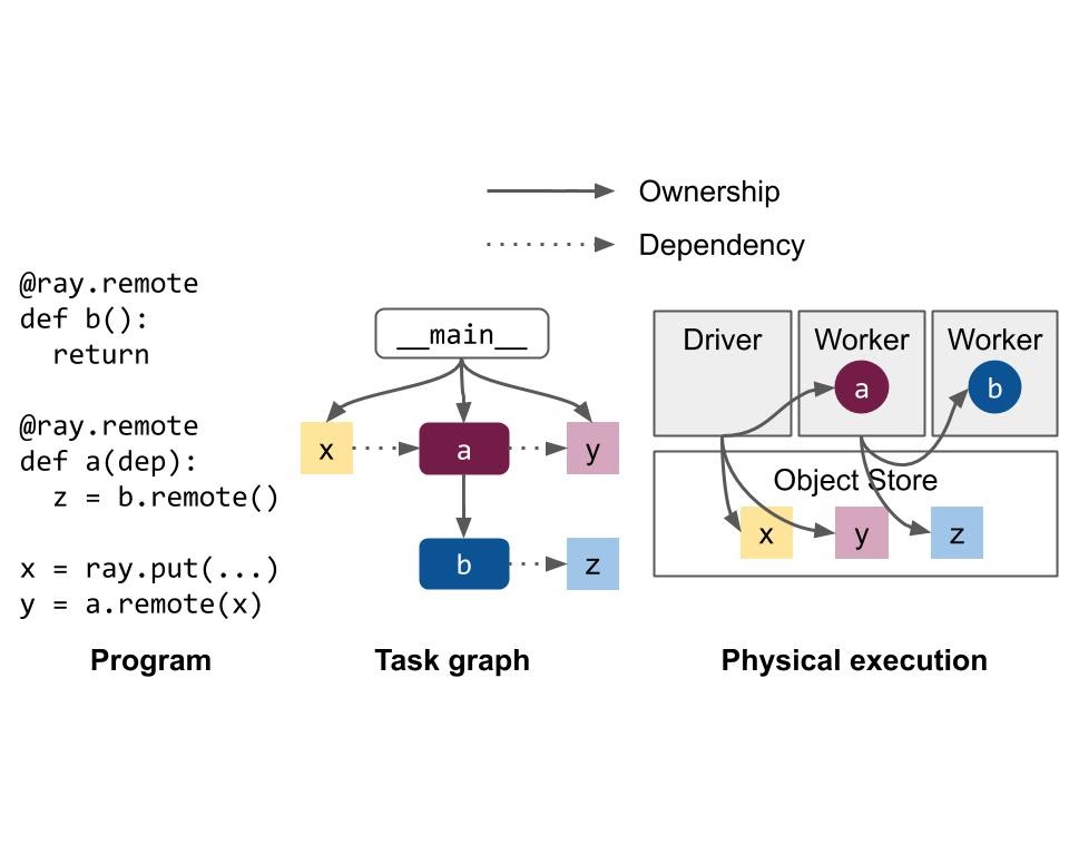
Most of the system metadata is managed according to a decentralized concept called ownership: Each worker process manages and owns the tasks that it submits and the ObjectRefs returned by those tasks. The owner is responsible for ensuring execution of the task and facilitating the resolution of an ObjectRef to its underlying value. Similarly, a worker owns any objects that it created through a ray.put call.
Lifetime of a Task
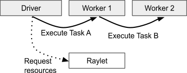
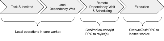
When a task is submitted, the owner waits for any dependencies, i.e. ObjectRefs that were passed as an argument to the task (see Lifetime of an Object), to become available. Note that the dependencies need not be local; the owner considers the dependencies to be ready as soon as they are available anywhere in the cluster. When the dependencies are ready, the owner requests resources from the distributed scheduler to execute the task. Once resources are available, the scheduler grants the request and responds with the address of a worker that is now leased to the owner.
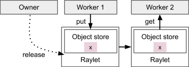
The owner schedules the task by sending the task specification over gRPC to the leased worker. After executing the task, the worker must store the return values. If the return values are small, the worker returns the values inline directly to the owner, which copies them to its in-process object store. If the return values are large, the worker stores the objects in its local shared memory store and replies to the owner indicating that the objects are now in distributed memory. This allows the owner to refer to the objects without having to fetch the objects to its local node.
When a task is submitted with an ObjectRef as its argument, the object value must be resolved before the worker can begin execution. If the value is small, it is copied directly from the owner’s in-process object store into the task description, where it can be referenced by the executing worker. If the value is large, the object must be fetched from distributed memory, so that the worker has a copy in its local shared memory store. The scheduler coordinates this object transfer by looking up the object’s locations and requesting a copy from a different node.
Lifetime of an Object
The owner of an object is the worker that created the initial ObjectRef, by submitting the creating task or calling ray.put. The owner manages the lifetime of the object. Ray guarantees that if the owner is alive, the object may eventually be resolved to its value (or an error is thrown in the case of worker failure). If the owner is dead, an attempt to get the object’s value will never hang but may throw an exception, even if there are still physical copies of the object.
Each worker stores a ref count for the objects that it owns. See Reference Counting for more information on how references are tracked. References are only counted during these operations:
- Passing an
ObjectRefor an object that contains anObjectRefas an argument to a task. - Returning an
ObjectRefor an object that contains anObjectReffrom a task.
Objects can be stored in the owner’s in-process memory store or in the distributed object store. This decision is meant to reduce the memory footprint and resolution time for each object.
Lifetime of an Actor
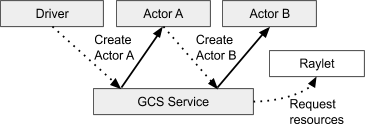
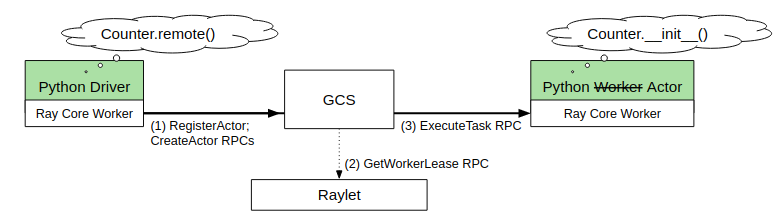
When an actor is created in Python, the creating worker first synchronously registers the actor with the GCS. This ensures correctness in case the creating worker fails before the actor can be created. Once the GCS responds, the remainder of the actor creation process is asynchronous. The creating worker process queues locally a special task known as the actor creation task. This is similar to a normal non-actor task, except that its specified resources are acquired for the lifetime of the actor process. The creator asynchronously resolves the dependencies for the actor creation task, then sends it to the GCS service to be scheduled. Meanwhile, the Python call to create the actor immediately returns an “actor handle” that can be used even if the actor creation task has not yet been scheduled. See Actor Creation for more details.
Task execution for actors is similar to that of normal tasks: they return futures, are submitted directly to the actor process via gRPC, and will not run until all ObjectRef dependencies have been resolved. There are two main differences:
- Resources do not need to be acquired from the scheduler to execute an actor task. This is because the actor has already been granted resources for its lifetime, when its creation task was scheduled.
- For each caller of an actor, the tasks are executed in the same order that they are submitted.
Object Management
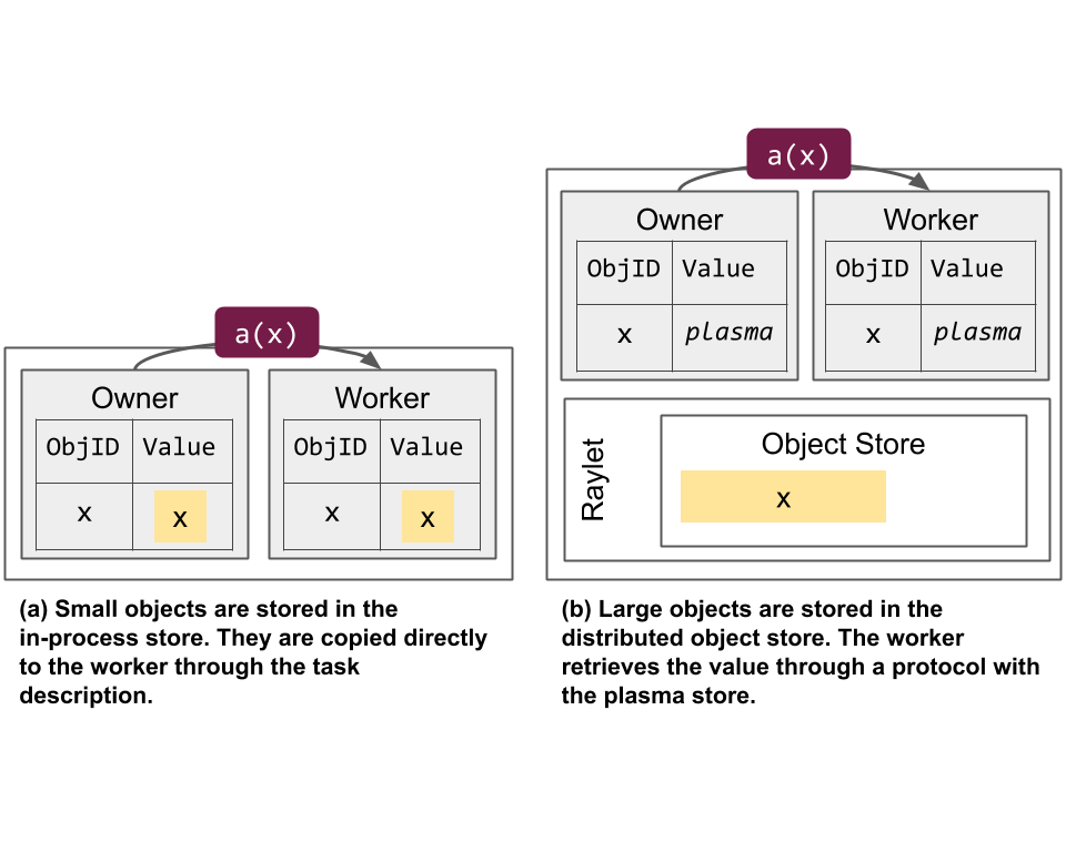
In general, small objects are stored in their owner’s in-process store while large objects are stored in the distributed object store. This decision is meant to reduce the memory footprint and resolution time for each object. Note that in the latter case, a placeholder object is stored in the in-process store to indicate the object has been promoted to shared memory.
Objects in the in-process store can be resolved quickly through a direct memory copy but may have a higher memory footprint when referenced by many processes due to the additional copies. The capacity of a single worker’s in-process store is also limited to the memory capacity of that machine, limiting the total number of such objects that can be in reference at any given time. For objects that are referenced many times, throughput may also be limited by the processing capacity of the owner process.
In contrast, resolution of an object in the distributed object store requires at least one IPC from the worker to the worker’s local shared memory store. Additional RPCs may be required if the worker’s local shared memory store does not yet contain a copy of the object. On the other hand, because the shared memory store is implemented with shared memory, multiple workers on the same node can reference the same copy of an object. This can reduce the overall memory footprint if an object can be deserialized with zero copies. The use of distributed memory also allows a process to reference an object without having the object local, meaning that a process can reference objects whose total size exceeds the memory capacity of a single machine. Finally, throughput can scale with the number of nodes in the distributed object store, as multiple copies of an object may be stored at different nodes.
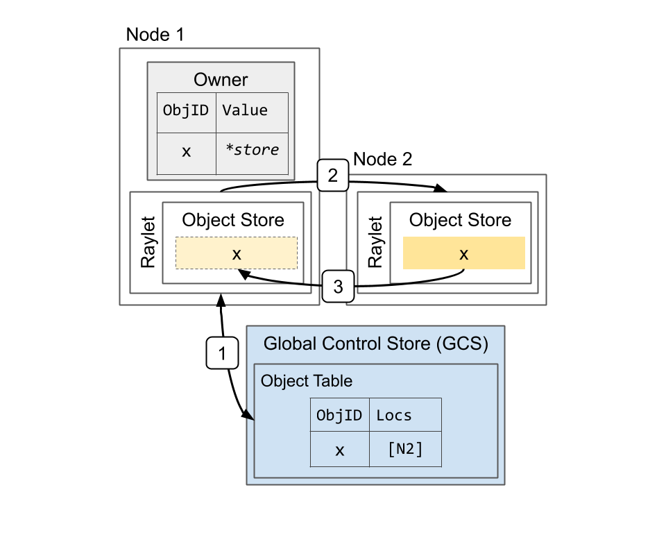
Resolving a large object. The object x is initially created on Node 2, e.g., because the task that returned the value ran on that node. This shows the steps when the owner (the caller of the task) calls ray.get: 1) Lookup object’s locations in the GCS. 2) Select a location and send a request for a copy of the object. 3) Receive the object.
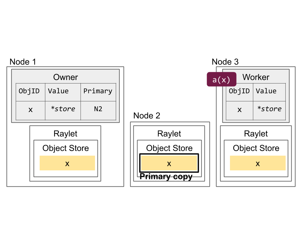
Primary copy versus evictable copies. The primary copy (Node 2) is ineligible for eviction. However, the copies on Nodes 1 (created through ray.get) and 3 (created through task submission) can be evicted under memory pressure.
Resource Management and Scheduling
A resource in Ray is any “key” -> float quantity. For convenience, the Ray scheduler has native support for CPU, GPU, and memory resource types, meaning that Ray automatically detects physical availability of these resources on each node. However, the user may also define custom resource requirements using any valid string, e.g., specifying a resource requirement of {“something”: 1}.
The owner waits for all task arguments to be created before requesting resources from the distributed scheduler. For example, for a program like foo.remote(bar.remote()), the owner will not schedule foo until bar has completed.
An owner schedules a task by first sending a resource request to its local raylet. The raylet queues the request and if it chooses to grant the resources, responds to the owner with the address of a local worker that is now leased to the owner. The lease remains active as long as the owner and leased worker are alive, and the raylet ensures that no other client may use the worker while the lease is active. To ensure fairness, an owner returns the worker if no work remains or if enough time has passed (e.g., a few hundred milliseconds).
Actor management
When an actor is created in Python, the creating worker first synchronously registers the actor with the GCS. This ensures that in the case that the creating worker dies before the actor can be created, any workers with a reference to the actor will be able to discover the failure.
Once all of the input dependencies for an actor creation task are resolved, the creator then sends the task specification to the GCS service. The GCS service then schedules the actor creation task through the same distributed scheduling protocol that is used for normal tasks, as if the GCS were the actor creation task’s owner. Because the GCS service persists all state to the backing store, once the task specification has successfully been sent to the GCS service, the actor will eventually be created.
[1] DistBelief: Large Scale Distributed Deep Networks
[3] Multiverso
[4] EASGD: Deep learning with Elastic Averaging SGD
[5] Hogwild!: A Lock-Free Approach to Parallelizing Stochastic Gradient Descent
[6] Cyclades: Conflict-free Asynchronous Machine Learning
[8] AdaDelay: Delay Adaptive Distributed Stochastic Convex Optimization
[9] Alexnet: ImageNet Classification with Deep Convolutional Neural Networks